This Jupyter notebook can be downloaded from rednoise-fit-example.ipynb, or viewed as a python script at rednoise-fit-example.py.
Red noise and DM noise fitting examples
This notebook provides an example on how to fit for red noise and DM noise using PINT using simulated datasets.
We will use the PLRedNoise and PLDMNoise models to generate noise realizations (these models provide Fourier Gaussian process descriptions of achromatic red noise and DM noise respectively).
We will fit the generated datasets using the WaveX and DMWaveX models, which provide deterministic Fourier representations of achromatic red noise and DM noise respectively.
Finally, we will convert the WaveX/DMWaveX amplitudes into spectral parameters and compare them with the injected values.
[1]:
from pint import DMconst
from pint.models import get_model
from pint.simulation import make_fake_toas_uniform
from pint.logging import setup as setup_log
from pint.fitter import WLSFitter
from pint.utils import (
    dmwavex_setup,
    find_optimal_nharms,
    wavex_setup,
    plrednoise_from_wavex,
    pldmnoise_from_dmwavex,
)

from io import StringIO
import numpy as np
import astropy.units as u
from matplotlib import pyplot as plt
from copy import deepcopy

setup_log(level="WARNING")
[1]:
1
Red noise fitting
Simulation
The first step is to generate a simulated dataset for demonstration. Note that we are adding PHOFF as a free parameter. This is required for the fit to work properly.
[2]:
par_sim = """
    PSR           SIM3
    RAJ           05:00:00     1
    DECJ          15:00:00     1
    PEPOCH        55000
    F0            100          1
    F1            -1e-15       1
    PHOFF         0            1
    DM            15           1
    TNREDAMP      -13
    TNREDGAM      3.5
    TNREDC        30
    TZRMJD        55000
    TZRFRQ        1400
    TZRSITE       gbt
    UNITS         TDB
    EPHEM         DE440
    CLOCK         TT(BIPM2019)
"""

m = get_model(StringIO(par_sim))
[3]:
# Now generate the simulated TOAs.
ntoas = 2000
toaerrs = np.random.uniform(0.5, 2.0, ntoas) * u.us
freqs = np.linspace(500, 1500, 8) * u.MHz

t = make_fake_toas_uniform(
    startMJD=53001,
    endMJD=57001,
    ntoas=ntoas,
    model=m,
    freq=freqs,
    obs="gbt",
    error=toaerrs,
    add_noise=True,
    add_correlated_noise=True,
    name="fake",
    include_bipm=True,
    include_gps=True,
    multi_freqs_in_epoch=True,
)
Optimal number of harmonics
The optimal number of harmonics can be estimated by minimizing the Akaike Information Criterion (AIC). This is implemented in the pint.utils.find_optimal_nharms function.
[4]:
m1 = deepcopy(m)
m1.remove_component("PLRedNoise")
nharm_opt, d_aics = find_optimal_nharms(m1, t, "WaveX", 30)
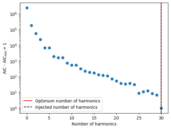
print("Optimum no of harmonics = ", nharm_opt)
Optimum no of harmonics = 10
[5]:
print(np.argmin(d_aics))
10
[6]:
# The Y axis is plotted in log scale only for better visibility.
plt.scatter(list(range(len(d_aics))), d_aics + 1)
plt.axvline(nharm_opt, color="red", label="Optimum number of harmonics")
plt.axvline(
    int(m.TNREDC.value), color="black", ls="--", label="Injected number of harmonics"
)
plt.xlabel("Number of harmonics")
plt.ylabel("AIC - AIC$_\\min{} + 1$")
plt.legend()
plt.yscale("log")
# plt.savefig("sim3-aic.pdf")
[7]:
# Now create a new model with the optimum number of harmonics
m2 = deepcopy(m1)
Tspan = t.get_mjds().max() - t.get_mjds().min()
wavex_setup(m2, T_span=Tspan, n_freqs=nharm_opt, freeze_params=False)

ftr = WLSFitter(t, m2)
ftr.fit_toas(maxiter=10)
m2 = ftr.model

print(m2)
# Created: 2024-03-05T20:42:14.731122
# PINT_version: 0.9.8+538.g1b3b20f
# User: docs
# Host: build-23657454-project-85767-nanograv-pint
# OS: Linux-5.19.0-1028-aws-x86_64-with-glibc2.35
# Python: 3.11.6 (main, Feb  1 2024, 16:47:41) [GCC 11.4.0]
# Format: pint
PSR                                  SIM3
EPHEM                               DE440
CLOCK                        TT(BIPM2019)
UNITS                                 TDB
START              53000.9999999568172454
FINISH             56985.0000000465657986
DILATEFREQ                              N
DMDATA                                  N
NTOA                                 2000
CHI2                   1963.0945922621618
CHI2R                  0.9949795196463059
TRES               0.98674543828378822317
RAJ                      4:59:59.99999853 1 0.00000124994340657381
DECJ                    14:59:59.99961532 1 0.00011558588454361496
PMRA                                  0.0
PMDEC                                 0.0
PX                                    0.0
F0                   99.99999999999982815 1 8.9973071726148309076e-14
F1              -9.999258178210027029e-16 1 3.2326809880527662077e-20
PEPOCH             55000.0000000000000000
TZRMJD             55000.0000000000000000
TZRSITE                               gbt
TZRFRQ                             1400.0
PHOFF              -0.0005341906008431784 1 0.00015978788860431827
PLANET_SHAPIRO                          N
DM                  14.999995690889103246 1 4.7825648357551326067e-06
WXEPOCH            55000.0000000000000000
WXFREQ_0001        0.00025100401605860257
WXSIN_0001         1.0083012455607141e-06 1 1.0360188118428624e-07
WXCOS_0001        -1.2549061794319808e-05 1 1.942509651578386e-06
WXFREQ_0002         0.0005020080321172051
WXSIN_0002         -2.725972143305833e-06 1 5.8413586245492664e-08
WXCOS_0002         3.7942271448721536e-06 1 4.880105240378557e-07
WXFREQ_0003         0.0007530120481758077
WXSIN_0003         1.5665929971713946e-06 1 4.5469342712024205e-08
WXCOS_0003         -4.188749004655945e-07 1 2.197840816039227e-07
WXFREQ_0004         0.0010040160642344103
WXSIN_0004         4.4849379355187464e-07 1 4.0265472970759674e-08
WXCOS_0004        -2.1166491485122707e-07 1 1.2722323032711892e-07
WXFREQ_0005         0.0012550200802930128
WXSIN_0005          8.733428411060071e-08 1 3.712723606765474e-08
WXCOS_0005         -1.108159627261607e-07 1 8.563047417279711e-08
WXFREQ_0006         0.0015060240963516154
WXSIN_0006        -1.4645278524275174e-07 1 3.5706467255575856e-08
WXCOS_0006          4.577088741014818e-08 1 6.404988330163363e-08
WXFREQ_0007          0.001757028112410218
WXSIN_0007         4.7754174372190335e-08 1 3.465330043901189e-08
WXCOS_0007         -1.705902843514892e-08 1 5.2474556632509865e-08
WXFREQ_0008         0.0020080321284688205
WXSIN_0008         2.4041321000948647e-08 1 3.396243579744871e-08
WXCOS_0008         1.0848646703320577e-07 1 4.582267135420585e-08
WXFREQ_0009         0.0022590361445274233
WXSIN_0009        -4.1125417691153365e-08 1 3.353509841014572e-08
WXCOS_0009         3.3177273801243306e-07 1 4.1415405011658896e-08
WXFREQ_0010         0.0025100401605860257
WXSIN_0010          5.124115614998029e-08 1 3.365652091377123e-08
WXCOS_0010         1.3334186572621743e-07 1 3.909490749026018e-08
Estimating the spectral parameters from the WaveX fit.
[8]:
# Get the Fourier amplitudes and powers and their uncertainties.
idxs = np.array(m2.components["WaveX"].get_indices())
a = np.array([m2[f"WXSIN_{idx:04d}"].quantity.to_value("s") for idx in idxs])
da = np.array([m2[f"WXSIN_{idx:04d}"].uncertainty.to_value("s") for idx in idxs])
b = np.array([m2[f"WXCOS_{idx:04d}"].quantity.to_value("s") for idx in idxs])
db = np.array([m2[f"WXCOS_{idx:04d}"].uncertainty.to_value("s") for idx in idxs])
print(len(idxs))

P = (a**2 + b**2) / 2
dP = ((a * da) ** 2 + (b * db) ** 2) ** 0.5

f0 = (1 / Tspan).to_value(u.Hz)
fyr = (1 / u.year).to_value(u.Hz)
10
[9]:
# We can create a `PLRedNoise` model from the `WaveX` model.
# This will estimate the spectral parameters from the `WaveX`
# amplitudes.
m3 = plrednoise_from_wavex(m2)
print(m3)
# Created: 2024-03-05T20:42:14.769746
# PINT_version: 0.9.8+538.g1b3b20f
# User: docs
# Host: build-23657454-project-85767-nanograv-pint
# OS: Linux-5.19.0-1028-aws-x86_64-with-glibc2.35
# Python: 3.11.6 (main, Feb  1 2024, 16:47:41) [GCC 11.4.0]
# Format: pint
PSR                                  SIM3
EPHEM                               DE440
CLOCK                        TT(BIPM2019)
UNITS                                 TDB
START              53000.9999999568172454
FINISH             56985.0000000465657986
DILATEFREQ                              N
DMDATA                                  N
NTOA                                 2000
CHI2                   1963.0945922621618
CHI2R                  0.9949795196463059
TRES               0.98674543828378822317
RAJ                      4:59:59.99999853 1 0.00000124994340657381
DECJ                    14:59:59.99961532 1 0.00011558588454361496
PMRA                                  0.0
PMDEC                                 0.0
PX                                    0.0
F0                   99.99999999999982815 1 8.9973071726148309076e-14
F1              -9.999258178210027029e-16 1 3.2326809880527662077e-20
PEPOCH             55000.0000000000000000
TZRMJD             55000.0000000000000000
TZRSITE                               gbt
TZRFRQ                             1400.0
PHOFF              -0.0005341906008431784 1 0.00015978788860431827
PLANET_SHAPIRO                          N
DM                  14.999995690889103246 1 4.7825648357551326067e-06
TNREDAMP              -13.064451842281922 0 0.1172632516393968
TNREDGAM                4.010525299130815 0 0.4386107990818431
TNREDC                               10.0
[10]:
# Now let us plot the estimated spectrum with the injected
# spectrum.
plt.subplot(211)
plt.errorbar(
    idxs * f0,
    b * 1e6,
    db * 1e6,
    ls="",
    marker="o",
    label="$\\hat{a}_j$ (WXCOS)",
    color="red",
)
plt.errorbar(
    idxs * f0,
    a * 1e6,
    da * 1e6,
    ls="",
    marker="o",
    label="$\\hat{b}_j$ (WXSIN)",
    color="blue",
)
plt.axvline(fyr, color="black", ls="dotted")
plt.axhline(0, color="grey", ls="--")
plt.ylabel("Fourier coeffs ($\mu$s)")
plt.xscale("log")
plt.legend(fontsize=8)

plt.subplot(212)
plt.errorbar(
    idxs * f0, P, dP, ls="", marker="o", label="Spectral power (PINT)", color="k"
)
P_inj = m.components["PLRedNoise"].get_noise_weights(t)[::2][:nharm_opt]
plt.plot(idxs * f0, P_inj, label="Injected Spectrum", color="r")
P_est = m3.components["PLRedNoise"].get_noise_weights(t)[::2][:nharm_opt]
print(len(idxs), len(P_est))
plt.plot(idxs * f0, P_est, label="Estimated Spectrum", color="b")
plt.xscale("log")
plt.yscale("log")
plt.ylabel("Spectral power (s$^2$)")
plt.xlabel("Frequency (Hz)")
plt.axvline(fyr, color="black", ls="dotted", label="1 yr$^{-1}$")
plt.legend()
10 10
[10]:
<matplotlib.legend.Legend at 0x7fc0118e6050>
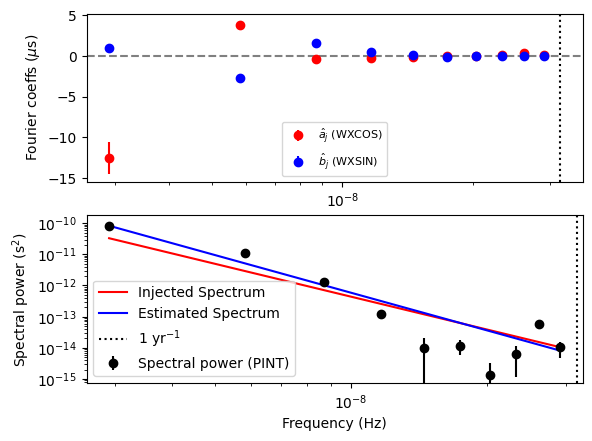
Note the outlier in the 1 year^-1 bin. This is caused by the covariance with RA and DEC, which introduce a delay with the same frequency.
DM noise fitting
Let us now do a similar kind of analysis for DM noise.
[11]:
par_sim = """
    PSR           SIM4
    RAJ           05:00:00     1
    DECJ          15:00:00     1
    PEPOCH        55000
    F0            100          1
    F1            -1e-15       1
    PHOFF         0            1
    DM            15           1
    TNDMAMP       -13
    TNDMGAM       3.5
    TNDMC         30
    TZRMJD        55000
    TZRFRQ        1400
    TZRSITE       gbt
    UNITS         TDB
    EPHEM         DE440
    CLOCK         TT(BIPM2019)
"""

m = get_model(StringIO(par_sim))
[12]:
# Generate the simulated TOAs.
ntoas = 2000
toaerrs = np.random.uniform(0.5, 2.0, ntoas) * u.us
freqs = np.linspace(500, 1500, 8) * u.MHz

t = make_fake_toas_uniform(
    startMJD=53001,
    endMJD=57001,
    ntoas=ntoas,
    model=m,
    freq=freqs,
    obs="gbt",
    error=toaerrs,
    add_noise=True,
    add_correlated_noise=True,
    name="fake",
    include_bipm=True,
    include_gps=True,
    multi_freqs_in_epoch=True,
)
[13]:
# Find the optimum number of harmonics by minimizing AIC.
m1 = deepcopy(m)
m1.remove_component("PLDMNoise")
m2 = deepcopy(m1)
nharm_opt, d_aics = find_optimal_nharms(m2, t, "DMWaveX", 30)
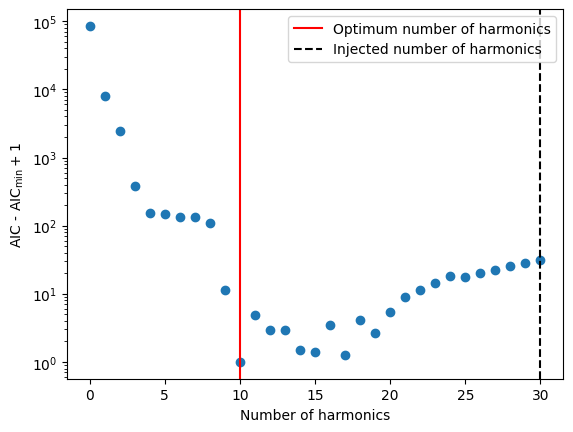
print("Optimum no of harmonics = ", nharm_opt)
Optimum no of harmonics = 30
[14]:
# The Y axis is plotted in log scale only for better visibility.
plt.scatter(list(range(len(d_aics))), d_aics + 1)
plt.axvline(nharm_opt, color="red", label="Optimum number of harmonics")
plt.axvline(
    int(m.TNDMC.value), color="black", ls="--", label="Injected number of harmonics"
)
plt.xlabel("Number of harmonics")
plt.ylabel("AIC - AIC$_\\min{} + 1$")
plt.legend()
plt.yscale("log")
# plt.savefig("sim3-aic.pdf")
[15]:
# Now create a new model with the optimum number of
# harmonics
m2 = deepcopy(m1)

Tspan = t.get_mjds().max() - t.get_mjds().min()
dmwavex_setup(m2, T_span=Tspan, n_freqs=nharm_opt, freeze_params=False)

ftr = WLSFitter(t, m2)
ftr.fit_toas(maxiter=10)
m2 = ftr.model

print(m2)
# Created: 2024-03-05T20:43:40.541355
# PINT_version: 0.9.8+538.g1b3b20f
# User: docs
# Host: build-23657454-project-85767-nanograv-pint
# OS: Linux-5.19.0-1028-aws-x86_64-with-glibc2.35
# Python: 3.11.6 (main, Feb  1 2024, 16:47:41) [GCC 11.4.0]
# Format: pint
PSR                                  SIM4
EPHEM                               DE440
CLOCK                        TT(BIPM2019)
UNITS                                 TDB
START              53000.9999999567961575
FINISH             56985.0000000473154514
DILATEFREQ                              N
DMDATA                                  N
NTOA                                 2000
CHI2                   1871.9921847836865
CHI2R                  0.9684387919212036
TRES               0.98394791313089790825
RAJ                      5:00:00.00000046 1 0.00000191447792630835
DECJ                    14:59:59.99983577 1 0.00016250048557228707
PMRA                                  0.0
PMDEC                                 0.0
PX                                    0.0
F0                  99.999999999999937675 1 3.6607242705813459093e-14
F1              -1.0000013051010914697e-15 1 8.441843540155421575e-22
PEPOCH             55000.0000000000000000
TZRMJD             55000.0000000000000000
TZRSITE                               gbt
TZRFRQ                             1400.0
PHOFF              -0.0018478067442315696 1 5.579379395389952e-06
PLANET_SHAPIRO                          N
DM                 15.0000040255508961225 1 5.0071694038580182972e-06
DMWXEPOCH          55000.0000000000000000
DMWXFREQ_0001        0.000251004016058554
DMWXSIN_0001       -0.0016535232742997381 1 6.071340859784536e-06
DMWXCOS_0001        -0.006142546716447953 1 6.933130992405707e-06
DMWXFREQ_0002        0.000502008032117108
DMWXSIN_0002       0.00039907056013591753 1 4.902042347474044e-06
DMWXCOS_0002       -0.0014433889713990897 1 4.52914159822426e-06
DMWXFREQ_0003        0.000753012048175662
DMWXSIN_0003        0.0005999679092541995 1 4.669986613406933e-06
DMWXCOS_0003       -0.0004605755161331775 1 4.339499479405041e-06
DMWXFREQ_0004        0.001004016064234216
DMWXSIN_0004       -9.523651370033758e-05 1 4.555259203390117e-06
DMWXCOS_0004       -0.0005331671746853744 1 4.30117992198666e-06
DMWXFREQ_0005         0.00125502008029277
DMWXSIN_0005       -6.579081736729088e-06 1 4.403757544329701e-06
DMWXCOS_0005        6.320791228219422e-06 1 4.405657480293348e-06
DMWXFREQ_0006        0.001506024096351324
DMWXSIN_0006       -0.0002727273462380033 1 4.407544324159355e-06
DMWXCOS_0006       -0.0001140184323825167 1 4.384510474010537e-06
DMWXFREQ_0007        0.001757028112409878
DMWXSIN_0007       5.9901161334588404e-05 1 4.374752975512751e-06
DMWXCOS_0007       -4.803408807250036e-05 1 4.394931479658995e-06
DMWXFREQ_0008        0.002008032128468432
DMWXSIN_0008      -1.3121820906063507e-05 1 4.446610129006186e-06
DMWXCOS_0008      -2.2799148132382645e-05 1 4.3384316792256065e-06
DMWXFREQ_0009       0.0022590361445269857
DMWXSIN_0009       0.00010234017218909656 1 4.36967730972814e-06
DMWXCOS_0009         6.75915793438724e-05 1 4.410292427981286e-06
DMWXFREQ_0010         0.00251004016058554
DMWXSIN_0010       -5.770568216228033e-05 1 4.417678428608208e-06
DMWXCOS_0010      -1.7929775636169557e-05 1 4.424463480860475e-06
DMWXFREQ_0011       0.0027610441766440937
DMWXSIN_0011        6.498793707240834e-06 1 7.136311833449328e-06
DMWXCOS_0011       2.3659681364342035e-05 1 6.9431739432001385e-06
DMWXFREQ_0012        0.003012048192702648
DMWXSIN_0012       -6.122050461292383e-05 1 4.3496916164214075e-06
DMWXCOS_0012      -2.1167917406272713e-05 1 4.46769237723148e-06
DMWXFREQ_0013       0.0032630522087612017
DMWXSIN_0013      -3.3280080996376774e-05 1 4.473355703481371e-06
DMWXCOS_0013       1.6522110158486613e-05 1 4.307751651177666e-06
DMWXFREQ_0014        0.003514056224819756
DMWXSIN_0014      -2.0987774486957135e-06 1 4.4205130778274e-06
DMWXCOS_0014       2.8026173021012704e-05 1 4.338297820443293e-06
DMWXFREQ_0015       0.0037650602408783097
DMWXSIN_0015       -9.197585474617963e-06 1 4.397118574288681e-06
DMWXCOS_0015      -1.6525289148640695e-05 1 4.363551381908189e-06
DMWXFREQ_0016        0.004016064256936864
DMWXSIN_0016        2.145607902192326e-05 1 4.336122939780618e-06
DMWXCOS_0016      -1.3076240214737695e-05 1 4.422727592619873e-06
DMWXFREQ_0017        0.004267068272995418
DMWXSIN_0017        4.927468719247008e-06 1 4.454091022977341e-06
DMWXCOS_0017       1.4251894402981327e-05 1 4.300209626069207e-06
DMWXFREQ_0018       0.0045180722890539714
DMWXSIN_0018      -1.6475185426847756e-05 1 4.221588824239981e-06
DMWXCOS_0018        7.264216000048718e-06 1 4.528641951156254e-06
DMWXFREQ_0019        0.004769076305112526
DMWXSIN_0019      -2.6139008904700963e-05 1 4.338153464698542e-06
DMWXCOS_0019       -6.440318310436699e-06 1 4.411935898365397e-06
DMWXFREQ_0020         0.00502008032117108
DMWXSIN_0020      -1.8416198531499903e-05 1 4.363870988429914e-06
DMWXCOS_0020       1.0844509265223118e-05 1 4.40124774625944e-06
DMWXFREQ_0021        0.005271084337229634
DMWXSIN_0021       2.2627972586933304e-05 1 4.448042074664561e-06
DMWXCOS_0021      -2.3840874704894125e-06 1 4.318704951444386e-06
DMWXFREQ_0022        0.005522088353288187
DMWXSIN_0022      -1.0783559764463234e-05 1 4.45130746849293e-06
DMWXCOS_0022        6.027636500472184e-07 1 4.310930991408283e-06
DMWXFREQ_0023        0.005773092369346741
DMWXSIN_0023       2.6849694088064136e-06 1 4.420265068655117e-06
DMWXCOS_0023      -1.0498684966956433e-06 1 4.331575010419854e-06
DMWXFREQ_0024        0.006024096385405296
DMWXSIN_0024        8.976205013394534e-06 1 4.325176231053102e-06
DMWXCOS_0024      -1.1761183680634569e-05 1 4.428323301874858e-06
DMWXFREQ_0025         0.00627510040146385
DMWXSIN_0025       1.5550249637889528e-05 1 4.503221327875144e-06
DMWXCOS_0025       1.6469761341054502e-05 1 4.24472211898906e-06
DMWXFREQ_0026        0.006526104417522403
DMWXSIN_0026       1.7693721611377547e-06 1 4.388676379961913e-06
DMWXCOS_0026       5.1114454764427425e-06 1 4.3520478320489355e-06
DMWXFREQ_0027        0.006777108433580957
DMWXSIN_0027        2.229518402299213e-06 1 4.3476436914472765e-06
DMWXCOS_0027       -6.945019518511143e-06 1 4.397576539163481e-06
DMWXFREQ_0028        0.007028112449639512
DMWXSIN_0028      -1.0438088402517298e-05 1 4.370306899754738e-06
DMWXCOS_0028        6.661910183051581e-06 1 4.381672217449315e-06
DMWXFREQ_0029        0.007279116465698066
DMWXSIN_0029        9.835116963803858e-06 1 4.363120544299024e-06
DMWXCOS_0029      -1.3179257476402031e-07 1 4.37831882557006e-06
DMWXFREQ_0030        0.007530120481756619
DMWXSIN_0030       -9.829436982073473e-06 1 4.37227802239831e-06
DMWXCOS_0030       -9.279896448510335e-06 1 4.368700336769009e-06
Estimating the spectral parameters from the DMWaveX fit.
[16]:
# Get the Fourier amplitudes and powers and their uncertainties.
# Note that the `DMWaveX` amplitudes have the units of DM.
# We multiply them by a constant factor to convert them to dimensions
# of time so that they are consistent with `PLDMNoise`.
scale = DMconst / (1400 * u.MHz) ** 2

idxs = np.array(m2.components["DMWaveX"].get_indices())
a = np.array(
    [(scale * m2[f"DMWXSIN_{idx:04d}"].quantity).to_value("s") for idx in idxs]
)
da = np.array(
    [(scale * m2[f"DMWXSIN_{idx:04d}"].uncertainty).to_value("s") for idx in idxs]
)
b = np.array(
    [(scale * m2[f"DMWXCOS_{idx:04d}"].quantity).to_value("s") for idx in idxs]
)
db = np.array(
    [(scale * m2[f"DMWXCOS_{idx:04d}"].uncertainty).to_value("s") for idx in idxs]
)
print(len(idxs))

P = (a**2 + b**2) / 2
dP = ((a * da) ** 2 + (b * db) ** 2) ** 0.5

f0 = (1 / Tspan).to_value(u.Hz)
fyr = (1 / u.year).to_value(u.Hz)
30
[17]:
# We can create a `PLDMNoise` model from the `DMWaveX` model.
# This will estimate the spectral parameters from the `DMWaveX`
# amplitudes.
m3 = pldmnoise_from_dmwavex(m2)
print(m3)
# Created: 2024-03-05T20:43:40.598359
# PINT_version: 0.9.8+538.g1b3b20f
# User: docs
# Host: build-23657454-project-85767-nanograv-pint
# OS: Linux-5.19.0-1028-aws-x86_64-with-glibc2.35
# Python: 3.11.6 (main, Feb  1 2024, 16:47:41) [GCC 11.4.0]
# Format: pint
PSR                                  SIM4
EPHEM                               DE440
CLOCK                        TT(BIPM2019)
UNITS                                 TDB
START              53000.9999999567961575
FINISH             56985.0000000473154514
DILATEFREQ                              N
DMDATA                                  N
NTOA                                 2000
CHI2                   1871.9921847836865
CHI2R                  0.9684387919212036
TRES               0.98394791313089790825
RAJ                      5:00:00.00000046 1 0.00000191447792630835
DECJ                    14:59:59.99983577 1 0.00016250048557228707
PMRA                                  0.0
PMDEC                                 0.0
PX                                    0.0
F0                  99.999999999999937675 1 3.6607242705813459093e-14
F1              -1.0000013051010914697e-15 1 8.441843540155421575e-22
PEPOCH             55000.0000000000000000
TZRMJD             55000.0000000000000000
TZRSITE                               gbt
TZRFRQ                             1400.0
PHOFF              -0.0018478067442315696 1 5.579379395389952e-06
PLANET_SHAPIRO                          N
DM                 15.0000040255508961225 1 5.0071694038580182972e-06
TNDMAMP               -13.007975991712817 0 0.044221629286904034
TNDMGAM                3.9217931261809316 0 0.23371136077496144
TNDMC                                30.0
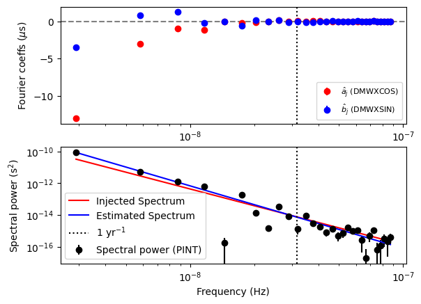
[18]:
# Now let us plot the estimated spectrum with the injected
# spectrum.
plt.subplot(211)
plt.errorbar(
    idxs * f0,
    b * 1e6,
    db * 1e6,
    ls="",
    marker="o",
    label="$\\hat{a}_j$ (DMWXCOS)",
    color="red",
)
plt.errorbar(
    idxs * f0,
    a * 1e6,
    da * 1e6,
    ls="",
    marker="o",
    label="$\\hat{b}_j$ (DMWXSIN)",
    color="blue",
)
plt.axvline(fyr, color="black", ls="dotted")
plt.axhline(0, color="grey", ls="--")
plt.ylabel("Fourier coeffs ($\mu$s)")
plt.xscale("log")
plt.legend(fontsize=8)

plt.subplot(212)
plt.errorbar(
    idxs * f0, P, dP, ls="", marker="o", label="Spectral power (PINT)", color="k"
)
P_inj = m.components["PLDMNoise"].get_noise_weights(t)[::2][:nharm_opt]
plt.plot(idxs * f0, P_inj, label="Injected Spectrum", color="r")
P_est = m3.components["PLDMNoise"].get_noise_weights(t)[::2][:nharm_opt]
print(len(idxs), len(P_est))
plt.plot(idxs * f0, P_est, label="Estimated Spectrum", color="b")
plt.xscale("log")
plt.yscale("log")
plt.ylabel("Spectral power (s$^2$)")
plt.xlabel("Frequency (Hz)")
plt.axvline(fyr, color="black", ls="dotted", label="1 yr$^{-1}$")
plt.legend()
30 30
[18]:
<matplotlib.legend.Legend at 0x7fc0044dadd0>