This Jupyter notebook can be downloaded from noise-fitting-example.ipynb, or viewed as a python script at noise-fitting-example.py.
PINT Noise Fitting Examples
[1]:
from pint.models import get_model
from pint.simulation import make_fake_toas_uniform
from pint.logging import setup as setup_log
from pint.fitter import Fitter

import numpy as np
from io import StringIO
from astropy import units as u
from matplotlib import pyplot as plt
[2]:
setup_log(level="WARNING")
[2]:
1
Fitting for EFAC and EQUAD
[3]:
# Let us begin by simulating a dataset with an EFAC and an EQUAD.
# Note that the EFAC and the EQUAD are set as fit parameters ("1").
par = """
    PSR             TEST1
    RAJ             05:00:00    1
    DECJ            15:00:00    1
    PEPOCH          55000
    F0              100         1
    F1              -1e-15      1
    EFAC tel gbt    1.3         1
    EQUAD tel gbt   1.1         1
    TZRMJD          55000
    TZRFRQ          1400
    TZRSITE         gbt
    EPHEM           DE440
    CLOCK           TT(BIPM2019)
    UNITS           TDB
"""

m = get_model(StringIO(par))

ntoas = 200

# EFAC and EQUAD cannot be measured separately if all TOA uncertainties
# are the same. So we must set a different toa uncertainty for each TOA.
# This is how it is in real datasets anyway.
toaerrs = np.random.uniform(0.5, 2, ntoas) * u.us

t = make_fake_toas_uniform(
    startMJD=54000,
    endMJD=56000,
    ntoas=ntoas,
    model=m,
    obs="gbt",
    error=toaerrs,
    add_noise=True,
    include_bipm=True,
    include_gps=True,
)
[4]:
# Now create the fitter. The `Fitter.auto()` function creates a
# Downhill fitter. Noise parameter fitting is only available in
# Downhill fitters.
ftr = Fitter.auto(t, m)
[5]:
# Now do the fitting.
ftr.fit_toas()
[6]:
# Print the post-fit model. We can see that the EFAC and EQUAD have been
# and the uncertainties are listed.
print(ftr.model)
# Created: 2024-03-05T20:40:40.754914
# PINT_version: 0.9.8+538.g1b3b20f
# User: docs
# Host: build-23657454-project-85767-nanograv-pint
# OS: Linux-5.19.0-1028-aws-x86_64-with-glibc2.35
# Python: 3.11.6 (main, Feb 1 2024, 16:47:41) [GCC 11.4.0]
# Format: pint
PSR TEST1
EPHEM DE440
CLOCK TT(BIPM2019)
UNITS TDB
START 53999.9999999864620718
FINISH 56000.0000000058119444
DILATEFREQ N
DMDATA N
NTOA 200
CHI2 199.99999873266935
CHI2R 1.0362694234853334
TRES 2.1024201282350863332
RAJ 5:00:00.00000714 1 0.00000759056552678821
DECJ 14:59:59.99911287 1 0.00066083327075091517
PMRA 0.0
PMDEC 0.0
PX 0.0
F0 100.00000000000005744 1 2.9438328721167584076e-13
F1 -9.9999540802219413085e-16 1 1.3591658847915768755e-20
PEPOCH 55000.0000000000000000
TZRMJD 55000.0000000000000000
TZRSITE gbt
TZRFRQ 1400.0
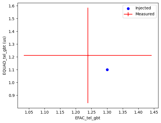
EFAC tel gbt 1.2383144859167698 1 0.20418100288170962
EQUAD tel gbt 1.2122076561435413 1 0.37362708996177063
PLANET_SHAPIRO N
[7]:
# Let us plot the injected and measured noise parameters together to
# compare them.
plt.scatter(m.EFAC1.value, m.EQUAD1.value, label="Injected", marker="o", color="blue")
plt.errorbar(
    ftr.model.EFAC1.value,
    ftr.model.EQUAD1.value,
    xerr=ftr.model.EFAC1.uncertainty_value,
    yerr=ftr.model.EQUAD1.uncertainty_value,
    marker="+",
    label="Measured",
    color="red",
)
plt.xlabel("EFAC_tel_gbt")
plt.ylabel("EQUAD_tel_gbt (us)")
plt.legend()
plt.show()
Fitting for ECORRs
[8]:
# Note the explicit offset (PHOFF) in the par file below.
# Implicit offset subtraction is typically not accurate enough when
# ECORR (or any other type of correlated noise) is present.
# i.e., PHOFF should be a free parameter when ECORRs are being fit.
par = """
    PSR             TEST2
    RAJ             05:00:00    1
    DECJ            15:00:00    1
    PEPOCH          55000
    F0              100         1
    F1              -1e-15      1
    PHOFF           0           1
    EFAC tel gbt    1.3         1
    ECORR tel gbt   1.1         1
    TZRMJD          55000
    TZRFRQ          1400
    TZRSITE         gbt
    EPHEM           DE440
    CLOCK           TT(BIPM2019)
    UNITS           TDB
"""

m = get_model(StringIO(par))

# ECORRs only apply when there are multiple TOAs per epoch.
# This can be simulated by providing multiple frequencies and
# setting the `multi_freqs_in_epoch` option. The `add_correlated_noise`
# option should also be set because correlated noise components
# are not simulated by default.

ntoas = 500
toaerrs = np.random.uniform(0.5, 2, ntoas) * u.us
freqs = np.linspace(1300, 1500, 4) * u.MHz

t = make_fake_toas_uniform(
    startMJD=54000,
    endMJD=56000,
    ntoas=ntoas,
    model=m,
    obs="gbt",
    error=toaerrs,
    freq=freqs,
    add_noise=True,
    add_correlated_noise=True,
    include_bipm=True,
    include_gps=True,
    multi_freqs_in_epoch=True,
)
[9]:
ftr = Fitter.auto(t, m)
[10]:
ftr.fit_toas()
[10]:
True
[11]:
print(ftr.model)
# Created: 2024-03-05T20:40:58.974207
# PINT_version: 0.9.8+538.g1b3b20f
# User: docs
# Host: build-23657454-project-85767-nanograv-pint
# OS: Linux-5.19.0-1028-aws-x86_64-with-glibc2.35
# Python: 3.11.6 (main, Feb 1 2024, 16:47:41) [GCC 11.4.0]
# Format: pint
PSR TEST2
EPHEM DE440
CLOCK TT(BIPM2019)
UNITS TDB
START 53999.9999999862346413
FINISH 55984.0000000565596759
DILATEFREQ N
DMDATA N
NTOA 500
CHI2 499.99576816641974
CHI2R 1.0162515613138612
TRES 1.6938202602025750443
RAJ 4:59:59.99999614 1 0.00000596934996562267
DECJ 14:59:59.99996079 1 0.00051011402458993554
PMRA 0.0
PMDEC 0.0
PX 0.0
F0 99.99999999999948706 1 2.3160754239197527554e-13
F1 -1.0000023319331419726e-15 1 1.0596442219069626431e-20
PEPOCH 55000.0000000000000000
TZRMJD 55000.0000000000000000
TZRSITE gbt
TZRFRQ 1400.0
PHOFF -2.47529919766377e-05 1 1.754787560413772e-05
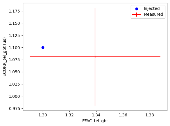
EFAC tel gbt 1.3391249958558036 1 0.04902198557247707
ECORR tel gbt 1.0810509877781542 1 0.10042212570888197
PLANET_SHAPIRO N
[12]:
# Let us plot the injected and measured noise parameters together to
# compare them.
plt.scatter(m.EFAC1.value, m.ECORR1.value, label="Injected", marker="o", color="blue")
plt.errorbar(
    ftr.model.EFAC1.value,
    ftr.model.ECORR1.value,
    xerr=ftr.model.EFAC1.uncertainty_value,
    yerr=ftr.model.ECORR1.uncertainty_value,
    marker="+",
    label="Measured",
    color="red",
)
plt.xlabel("EFAC_tel_gbt")
plt.ylabel("ECORR_tel_gbt (us)")
plt.legend()
plt.show()